Correlation refers to the idea that two variables (x and y) impact each other. For instance, the grades in a statistics class may be related to, or correlated with the amount of time those students study. As study time goes up, grades go up. This would be a positive correlation. On the other hand, as time spent partying, grades go down. This is called a negative correlation.
A positive correlation doesn’t strictly refer to good things, though. As the percent of poverty in a community goes up, the amount of crime may also go up. This is a positive correlation, but certainly not a good thing!
Correlations are expressed from -1 (which is perfectly negative) and +1 (which is perfectly positive.) The number shows the strength, and the sign (positive or negative) shows the direction. Therefore, -0.75 is a stronger correlation (or connection) than 0.25.
One common expression is “Correlation is not causation”; this refers to the idea that items can be correlated without really being related to each other. For instance, there is a close connection between the rates of ice-cream consumption in the winter and the drowning rate, even though one really doesn’t affect the other.
How to Calculate Correlation
Pearson’s r (also known as the correlation coefficient) is a simple correlation tool to work with. (Technically the r is used for samples and p is used for populations, but we’ll be working with samples, a limited amount of the total so we will simply refer to it as Pearson’s r or r.)
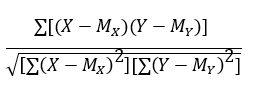
The formula is here:
This formula may look complicated, but let’s step through it step by step.
The sum of the values of X subtracted from the mean of X multipled by the values of Y subtracted from the mean of Y divided by the square root of X subtracted from the mean of X-squared multiplied by Y subtracted from the mean of Y-squared.
Let’s look at the following set of data of student absences and their final grades:
| Student # | Absences | Exam Grade |
| 1 | 4 | 82 |
| 2 | 2 | 98 |
| 3 | 2 | 76 |
| 4 | 3 | 68 |
| 5 | 1 | 84 |
| 6 | 0 | 99 |
| 7 | 4 | 67 |
| 8 | 8 | 58 |
| 9 | 7 | 50 |
| 10 | 3 | 78 |
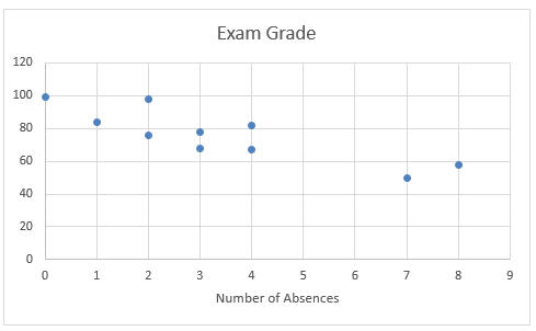
The first step is to create a scatterplot of the data to see if any patterns stick out:
This shows a moderately negative correlation, as absences go up, grades go down.
Moving to the equation, let’s look at the top part fist:
∑[(X-MX)(Y-MY)]
We have to calculate the mean of X and the mean of Y:
4 + 2 + 2 + 3 + 1 + 0 + 4 + 8 + 7 + 3 = 34 / 10 = Mean of X of 3.4
82 + 98 + 76 + 68 + 84 + 99 + 67 + 58 + 50 + 78 = 760 / 10 = Mean of Y of 76.
Next, we calculate X-Mx and Y-My, and sum them up.
| X | X – Mx | Y | Y – My |
| 4 | 0,6 | 82 | 6 |
| 2 | -1,4 | 98 | 22 |
| 2 | -1,4 | 76 | 0 |
| 3 | -0,4 | 68 | -8 |
| 1 | -2,4 | 84 | 8 |
| 0 | -3,4 | 99 | 23 |
| 4 | 0,6 | 67 | -9 |
| 8 | 4,6 | 58 | -18 |
| 7 | 3,6 | 50 | -26 |
| 3 | -0,4 | 78 | 2 |
Next, we must multiply the values of each of these together:
| X – Mx | Y – My | X-Mx * Y-My |
| 0,6 | 6 | 3,6 |
| -1,4 | 22 | -30,8 |
| -1,4 | 0 | 0 |
| -0,4 | -8 | 3,2 |
| -2,4 | 8 | -19,2 |
| -3,4 | 23 | -78,2 |
| 0,6 | -9 | -5,4 |
| 4,6 | -18 | -82,8 |
| 3,6 | -26 | -93,6 |
| -0,4 | 2 | -0,8 |
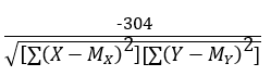
And the sum of these (3.6 + -30.8 + 0 + 3.2 and so on) is -304. Here’s our equation so far:
Next, let’s look at the bottom part of the equation:
| X | X – Mx | (X-Mx)2 | Y | Y – My | (Y-My)2 |
| 4 | 0,6 | 0.36 | 82 | 6 | 36 |
| 2 | -1,4 | 1.96 | 98 | 22 | 484 |
| 2 | -1,4 | 1.96 | 76 | 0 | 0 |
| 3 | -0,4 | 0.16 | 68 | -8 | 64 |
| 1 | -2,4 | 5.76 | 84 | 8 | 64 |
| 0 | -3,4 | 11.56 | 99 | 23 | 529 |
| 4 | 0,6 | 0.36 | 67 | -9 | 81 |
| 8 | 4,6 | 21.16 | 58 | -18 | 324 |
| 7 | 3,6 | 12.96 | 50 | -26 | 676 |
| 3 | -0,4 | 0.16 | 78 | 2 | 4 |
|
∑ |
56.4 |
∑ |
2262 | ||
We take the square of each of the X values and sum them up. We do the same for the Y values.
This results in: -304 / Sqrt(56.4*2262)
Next, we multiply the two bottoms together. 56.4 x 2262 = 127,576.8.
Taking the square root yields 357.179.
Our final calculation is -304 / 357.179 which equals -0.85.
-0.85 is our final correlation, which we can confirm using Excel’s CORREL function.
1 thought on “Correlation (Calculating Pearson’s r)”